
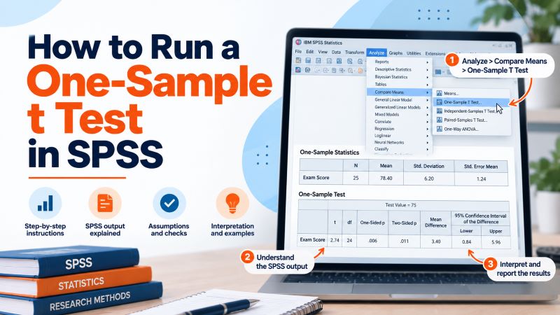
A one-sample t test compares the mean of one numerical variable with a specific known or hypothesized value. You might use it to determine whether the average exam score at a university differs from a national benchmark, whether average working hours differ from a specified standard, or whether a questionnaire score differs from a theoretical midpoint.
To run a one-sample t test in SPSS, go to Analyze > Compare Means > One-Sample T Test, move your numerical variable into the Test Variable(s) box, enter the comparison value in the Test Value box, and click OK.
Depending on your version of SPSS, the menu may appear as Analyze > Compare Means and Proportions > One-Sample T Test.
SPSS will then produce the sample mean, standard deviation, t statistic, degrees of freedom, p value, mean difference, and confidence interval. Recent versions can also calculate an effect size.
This guide walks through the complete process using one example, from choosing the correct test value to interpreting the final SPSS output.
When Should You Use a One-Sample t Test?
Use a one-sample t test when you have one sample, one numerical outcome, and one fixed comparison value.
The test answers a question such as:
Does the average exam score of these students differ from the national benchmark of 75?
The comparison value might represent:
- a national or industry benchmark;
- an established population value;
- a required standard;
- a theoretical value;
- a questionnaire midpoint;
- a value specified in your research hypothesis.
For example, suppose a researcher collects examination scores from 25 university students and wants to determine whether their mean score differs from a national benchmark of 75.
The researcher has:
One group: 25 students
One numerical variable: Exam score
One comparison value: 75
A one-sample t test fits this research question.
Do not use a one-sample t test when you want to compare two separate groups or two measurements from the same participants.
| Research question | Appropriate test |
|---|---|
| Does one sample mean differ from 75? | One-sample t test |
| Do male and female students have different mean scores? | Independent samples t test |
| Did the same students improve from pretest to posttest? | Paired samples t test |
Choosing the correct t test depends on your study design rather than the values in your dataset.
Example Used in This Guide
Suppose a researcher wants to know whether university students perform differently from a national examination benchmark of 75 points.
A sample of 25 students has the following descriptive statistics:
| Statistic | Value |
|---|---|
| Sample size, n | 25 |
| Mean, M | 78.40 |
| Standard deviation, SD | 6.20 |
| Test value | 75 |
The sample mean is 3.40 points above the benchmark:
78.40 − 75 = 3.40
However, this descriptive difference alone does not tell us whether the population mean differs statistically from 75.
The one-sample t test evaluates that question.
For a two-sided test, the hypotheses are:
H₀: μ = 75
H₁: μ ≠ 75
The null hypothesis states that the population mean equals 75. The alternative hypothesis states that the population mean differs from 75.
Assumptions of the One-Sample t Test
Before running the test, check whether a one-sample t test makes sense for your data.
Your Outcome Variable Should Be Numerical
The variable you test should represent meaningful numerical measurements, such as:
- examination scores;
- age;
- income;
- blood pressure;
- reaction time;
- height;
- scale or composite questionnaire scores.
Do not run a one-sample t test on participant IDs or category codes simply because SPSS stores them as numbers.
For example, a variable coded as:
1 = Male
2 = Female
remains categorical and does not meet the purpose of a one-sample t test.
Observations Should Be Independent
Each observation should contribute independently to the analysis.
For example, if every row represents a different student and each student contributes one exam score, the observations may reasonably satisfy this condition.
If you have repeated measurements from the same participants, consider whether a paired design better reflects your research question.
Check for Serious Outliers
A one-sample t test focuses on the sample mean, so extreme observations can have a large effect on the result.
Check for obvious data-entry errors and unusually extreme observations before running the test.
Do not automatically delete a value simply because it looks unusual. First determine whether the value represents an error, a genuine observation, or a feature of the population you are studying.
Consider the Distribution
The one-sample t test assumes that the outcome follows an approximately normal distribution in the population.
The test often tolerates moderate departures from normality, particularly with larger samples. However, strong skewness and extreme outliers deserve closer attention, especially with a small sample.
Before running the t test, it helps to inspect your variable using descriptive statistics and appropriate plots.
Our guide on How to Run Descriptive Statistics in SPSS shows how to examine the mean, standard deviation, minimum, maximum, and distribution of a variable before conducting further analysis.
How to Run a One-Sample t Test in SPSS
Once your data meet the requirements of the test, you can run the analysis in a few steps.
Step 1: Check Your Data Setup
Your dataset should contain one row for each observation and one column for the numerical variable you want to test.
For our example, the dataset contains a variable named:
Exam_Score
Each row contains the examination score for one student.
You do not need to create another variable containing the benchmark value of 75. SPSS lets you enter that fixed value directly when you run the test.
Before continuing, check that the variable contains the values you expect and that SPSS recognizes it as a numerical variable.
Step 2: Open the One-Sample T Test Dialog Box
From the main SPSS menu, go to:
Analyze > Compare Means > One-Sample T Test
Some versions display the procedure under:
Analyze > Compare Means and Proportions > One-Sample T Test
SPSS will open the One-Sample T Test dialog box.
You will see your variables on the left and a Test Variable(s) box on the right.
Step 3: Select the Test Variable
Select the numerical variable that contains the observations you want to test.
For this example, select:
Exam_Score
Move it into the Test Variable(s) box.
Make sure you select the actual numerical outcome rather than an ID number, category code, or unrelated variable.
SPSS allows you to place several variables in this box. It will run a separate one-sample t test for each variable against the same test value.
For a straightforward analysis, however, testing one outcome at a time often makes the output easier to follow.
Step 4: Enter the Test Value
Locate the Test Value field.
Enter:
75
This value represents the population mean specified by the null hypothesis.
SPSS will compare your sample mean with 75.
For our example:
Sample mean = 78.40
Test value = 75
The observed mean difference is therefore:
78.40 − 75 = 3.40
A crucial point is that the test value should come from your research question or a defensible benchmark.
Do not experiment with several test values until one produces a significant result.
Step 5: Review the Options
Click Options.
SPSS normally uses a 95% confidence interval. For a conventional two-sided test with α = .05, you would usually keep this setting.
The Options window may also allow you to control how SPSS handles missing values when you test several variables.
If your version provides an Estimate effect sizes option, select it when you want SPSS to calculate standardized effect sizes such as Cohen’s d.
Click Continue after reviewing the settings.
Step 6: Run the Test
Click OK.
SPSS will send the results to the Output Viewer.
For a basic one-sample t test, focus on these tables:
- One-Sample Statistics
- One-Sample Test
If you requested effect sizes, SPSS may also produce an effect-size table.
How to Interpret the One-Sample Statistics Table
The One-Sample Statistics table provides descriptive information about your sample.
For our example, suppose SPSS reports:
| Variable | N | Mean | Std. Deviation | Std. Error Mean |
|---|---|---|---|---|
| Exam Score | 25 | 78.40 | 6.20 | 1.24 |
Start with these values before interpreting statistical significance.
N
N = 25 tells us that SPSS included 25 valid observations in the test.
Check this value against the number of cases you expected.
If you expected 30 observations but SPSS reports 25, investigate whether missing values, filters, or data-entry problems reduced the sample.
Mean
The sample mean is:
M = 78.40
The students therefore scored an average of 78.40 points.
Since the test value is 75, the sample mean lies 3.40 points above the benchmark.
Standard Deviation
The standard deviation is:
SD = 6.20
This statistic describes the spread of the exam scores around their sample mean.
Standard Error Mean
SPSS reports:
SE = 1.24
The standard error describes the estimated sampling variability of the sample mean.
For a one-sample t test, SPSS calculates it from the sample standard deviation and sample size:
SE = SD / √n
For this example:
6.20 / √25 = 1.24
The t statistic compares the observed mean difference with this standard error.
How to Interpret the One-Sample Test Table
The One-Sample Test table contains the main hypothesis-test results.
For our example, the results are approximately:
| Statistic | Result |
|---|---|
| Test value | 75 |
| t | 2.74 |
| df | 24 |
| Two-sided p | .011 |
| Mean Difference | 3.40 |
| 95% CI of the Difference | [0.84, 5.96] |
Each value tells you something different about the result.
t Statistic
The t statistic is:
t = 2.74
The test statistic represents the observed mean difference relative to its standard error.
Conceptually:
t = (Sample mean − Test value) / Standard error
For our example:
t = (78.40 − 75) / 1.24
= 3.40 / 1.24
≈ 2.74
A positive t statistic means that the sample mean is above the test value. A negative t statistic means that the sample mean is below the test value.
The sign alone does not tell you whether the result reaches statistical significance.
Degrees of Freedom
SPSS reports:
df = 24
For a one-sample t test:
df = n − 1
Therefore:
25 − 1 = 24
The degrees of freedom help determine the reference t distribution that SPSS uses to calculate the p value and confidence interval.
p Value
For our example:
p = .011
Our two-sided alternative hypothesis asks whether the population mean differs from 75.
Using α = .05:
.011 < .05
The result is statistically significant.
We therefore reject the null hypothesis that the population mean equals 75 and conclude that the sample provides evidence that the population mean differs from the benchmark.
The sample mean also tells us the direction:
78.40 > 75
In this example, students scored higher on average than the benchmark.
Do not rely on the p value alone. Always look at the sample mean, mean difference, confidence interval, and effect size as well.
One-Sided vs. Two-Sided p Values in SPSS
Current SPSS output may display separate columns for:
One-Sided p
and:
Two-Sided p
Your research hypothesis determines which one you should use.
Use the two-sided p value when the alternative hypothesis asks whether the mean differs in either direction:
H₁: μ ≠ 75
This hypothesis allows the population mean to be either higher or lower than 75.
Use a one-sided test only when you specified a justified directional hypothesis before analyzing the data.
For example:
H₁: μ > 75
or:
H₁: μ < 75
Do not choose the one-sided p value simply because it gives you a smaller number after you have seen the results.
For our example, the question asks whether examination scores differ from 75, so the two-sided p value is appropriate.
Older versions of SPSS may label this result Sig. (2-tailed) instead.
What Does Mean Difference Mean in SPSS?
The Mean Difference often causes unnecessary confusion.
SPSS calculates it as:
Sample mean − Test value
In our example:
78.40 − 75 = 3.40
Therefore:
Mean Difference = 3.40
A positive mean difference tells you that the sample mean is higher than the test value.
A negative value tells you that the sample mean is lower.
For example, suppose your sample mean were 72 and the test value remained 75:
72 − 75 = −3
SPSS would report:
Mean Difference = −3.00
That negative sign does not indicate an error. It simply shows the direction of the difference.
How to Interpret the 95% Confidence Interval
For our example, SPSS reports a 95% confidence interval for the mean difference of approximately:
95% CI [0.84, 5.96]
This interval refers to the difference between the population mean and the test value.
It does not directly represent the confidence interval for the raw exam-score mean.
In our example, the complete interval lies above zero.
That result agrees with the significant two-sided t test because zero represents no difference from the benchmark.
If SPSS instead reported:
95% CI [−1.20, 4.30]
the interval would include zero. For a conventional two-sided test at α = .05, that would correspond to a nonsignificant result.
The confidence interval adds useful information because it shows the range of plausible values for the population mean difference under the model.
If you need a confidence interval for the population mean itself, add the test value to both confidence limits.
For our example:
Lower limit: 75 + 0.84 = 75.84
Upper limit: 75 + 5.96 = 80.96
This gives a corresponding 95% confidence interval for the population mean of approximately:
[75.84, 80.96]
How to Interpret Cohen’s d for a One-Sample t Test
Statistical significance tells you whether the data provide evidence against the null hypothesis. It does not tell you how large the difference is.
An effect size helps answer that second question.
If you request effect-size estimates in a recent version of SPSS, the software can calculate standardized effects for the t test.
For a basic one-sample Cohen’s d:
d = (Sample mean − Test value) / Sample standard deviation
Using our example:
d = (78.40 − 75) / 6.20
d ≈ 0.55
Researchers often use the following conventional reference points:
| Cohen’s d | Conventional description |
|---|---|
| 0.20 | Small |
| 0.50 | Medium |
| 0.80 | Large |
Treat these values as general reference points rather than rigid universal rules. The practical importance of an effect depends on the subject area, measurement scale, and research context.
For our example, d ≈ 0.55 represents a moderate standardized difference under these conventional guidelines.
The effect size therefore complements the p value rather than replacing it.
What If the One-Sample t Test Is Not Significant?
Suppose another analysis produces:
t(24) = 1.12, p = .274
Since:
.274 > .05
the result does not reach statistical significance at α = .05.
You would fail to reject the null hypothesis.
Do not conclude that you have proven the population mean equals the test value.
A nonsignificant result means that your sample does not provide sufficient evidence of a difference at the chosen significance level.
You should still examine the:
- sample mean;
- standard deviation;
- mean difference;
- confidence interval;
- effect size;
- sample size.
For example, a small study may produce an imprecise estimate even when the observed mean difference appears meaningful.
A nonsignificant result still represents a valid statistical finding.
Complete Interpretation of the Example
Our example produced the following results:
| Statistic | Result |
|---|---|
| Sample size | 25 |
| Sample mean | 78.40 |
| Standard deviation | 6.20 |
| Test value | 75 |
| Mean difference | 3.40 |
| t | 2.74 |
| df | 24 |
| Two-sided p | .011 |
| 95% CI of difference | [0.84, 5.96] |
| Cohen’s d | 0.55 |
The sample mean of 78.40 is 3.40 points above the benchmark of 75.
The one-sample t test produced t(24) = 2.74, p = .011. Since the p value falls below .05, the sample provides evidence that the population mean differs from 75.
Because the sample mean exceeds the benchmark, the observed difference points in the positive direction.
The 95% confidence interval for the difference, [0.84, 5.96], remains above zero and agrees with the statistically significant result.
Cohen’s d of approximately 0.55 suggests a moderate standardized difference according to conventional guidelines.
Together, these statistics provide a much fuller interpretation than the p value alone.
How to Run a One-Sample t Test Using SPSS Syntax
You can also run the test using SPSS syntax.
Suppose:
Variable = exam_score
Test value = 75
Use:
T-TEST
  /TESTVAL=75
  /VARIABLES=exam_score
  /CRITERIA=CI(.95).
This syntax tells SPSS to compare the mean of exam_score with 75 and calculate a 95% confidence interval.
You do not need syntax to perform the analysis correctly. The menu method works well for beginners.
However, syntax becomes especially useful for dissertations, theses, and larger research projects because it provides a reproducible record of your analysis.
You can rerun the same procedure after correcting data or updating the dataset without rebuilding every dialog box.
How to Report a One-Sample t Test
The main purpose of this guide is to help you run and understand the analysis, but you should know which statistics you will eventually need for your Results section.
For our example, a concise result could read:
Students had a mean examination score of 78.40 (SD = 6.20), which was significantly higher than the benchmark of 75, t(24) = 2.74, p = .011, 95% CI [0.84, 5.96], d = 0.55.
Notice that this sentence reports more than statistical significance.
It includes the:
- sample mean;
- standard deviation;
- benchmark;
- t statistic;
- degrees of freedom;
- p value;
- confidence interval;
- effect size.
When reporting the test in a formal paper, dissertation, or thesis, follow the formatting requirements of the style guide or institution you use.
Want to learn more about reporting the one-sample t test results? See our complete guide on how to report a one-sample t test in APA style.
Common Mistakes When Running a One-Sample t Test in SPSS
Several mistakes can lead to a technically correct SPSS calculation but an incorrect analysis or interpretation.
- Choosing an arbitrary test value. Use a benchmark that comes from your research question, theory, established standard, or another defensible source.
- Using the wrong type of t test. A one-sample t test compares one sample mean with one fixed value. It does not compare two groups.
- Testing a categorical variable. The test variable should represent meaningful numerical measurements.
- Confusing the test value with another sample. The test value is a fixed number, not a second group of observations.
- Ignoring extreme outliers. Extreme observations can substantially affect the mean, standard deviation, and t statistic.
- Looking only at the p value. Also examine the sample mean, mean difference, confidence interval, and effect size.
- Misinterpreting a negative t statistic. A negative t value generally means that the sample mean lies below the test value.
- Reporting p = .000. If SPSS displays
.000, report the result as p < .001, not p = .000. - Selecting a one-sided p value after seeing the data. Decide whether your hypothesis is directional before examining the result.
- Claiming that a nonsignificant result proves equality. Failure to reject the null hypothesis does not prove that the population mean exactly equals the test value.
- Calling a result significant because the sample mean looks different.
A descriptive difference does not automatically represent a statistically significant difference. - Copying the entire SPSS output into the Results section.
Select and report the statistics that your reader needs.
One-Sample t Test SPSS Checklist
Before you finish the analysis, check the following:
- Your outcome variable is numerical.
- Each observation contributes independently.
- The comparison value has a clear justification.
- You checked the data for errors and serious outliers.
- You considered the shape of the distribution.
- The N in SPSS matches the number of valid observations you expected.
- You know the sample mean and standard deviation.
- You understand how the sample mean compares with the test value.
- You identified the t statistic and degrees of freedom.
- You selected the correct one-sided or two-sided p-value.
- You interpreted the mean difference correctly.
- You checked whether the confidence interval includes zero.
- You considered the effect size where appropriate.
- You can explain the result without relying only on statistical significance.
If you can answer each of these points, you understand the analysis rather than simply knowing which SPSS buttons to click.
Need Help With Your One-Sample t Test in SPSS?
A one-sample t test becomes straightforward once you know what your test value represents and how to read each part of the SPSS output. The difficult part is often deciding whether the test fits your research question, checking the assumptions, and explaining what the result actually means.
If you are working with your own assignment, dissertation, thesis, or research dataset, you can work one-to-one with a tutor through spss-tutors.com.
Your tutor can guide you through the analysis using your own data, explain the SPSS output, and help you understand the statistical reasoning behind the test.
Frequently Asked Questions
What is a one-sample t test in SPSS?
A one-sample t test determines whether the mean of one numerical variable differs statistically from a specified value.
For example, you can test whether the mean examination score of a group of students differs from a benchmark of 75.
Where is the one-sample t test in SPSS?
Go to:
Analyze > Compare Means > One-Sample T Test
Depending on your SPSS version, you may see:
Analyze > Compare Means and Proportions > One-Sample T Test
What do I enter in the Test Value box?
Enter the fixed value that your null hypothesis specifies.
For example, if your research question asks whether the mean examination score differs from 75, enter:
75
The test value should come from the research question or another defensible benchmark rather than from trial and error.
What does Mean Difference mean in a one-sample t test?
SPSS calculates the mean difference as:
Sample mean − Test value
If the sample mean equals 78.40 and the test value equals 75:
Mean Difference = 3.40
A positive value means the sample mean is higher than the benchmark. A negative value means it is lower.
Which p value should I use for a one-sample t test in SPSS?
Use the two-sided p value when your alternative hypothesis asks whether the mean differs from the test value in either direction.
Use a one-sided p value only when you specified and justified a directional hypothesis before analyzing the data.
What does Sig. (2-tailed) mean in older SPSS output?
Older SPSS versions may label the two-sided p value as Sig. (2-tailed).
It tests whether the population mean differs from the test value in either direction.
What are the degrees of freedom for a one-sample t test?
For a one-sample t test:
df = n − 1
If your sample contains 25 valid observations:
df = 24
What does a negative t value mean?
A negative t statistic usually means the sample mean lies below the test value.
It does not automatically mean that the result is statistically significant or that the analysis is incorrect.
Check the p value and confidence interval before drawing a conclusion.
Does SPSS calculate Cohen’s d for a one-sample t test?
Recent versions of SPSS can calculate t-test effect sizes when you select the effect-size option.
If your version does not provide the estimate automatically, you can calculate one-sample Cohen’s d as:
d = (Sample mean − Test value) / Sample standard deviation
What should I do if p is greater than .05?
If the p value exceeds your significance level, you normally fail to reject the null hypothesis.
Do not say that you have proven the mean equals the test value. Instead, explain that the sample did not provide sufficient evidence of a difference at the chosen significance level.
Do I need to check normality before a one-sample t test?
You should consider the distribution of the outcome, particularly when your sample is small.
Look for strong skewness and serious outliers rather than expecting the sample to look perfectly normal. As sample sizes increase, the t test generally becomes more tolerant of moderate departures from normality, although influential outliers can still cause problems.
Can I use a one-sample t test with Likert-scale data?
It depends on what your variable represents.
A single Likert item is ordinal and may not suit a one-sample t test. Researchers sometimes analyze composite scores created from multiple Likert items as scale variables, depending on the measurement properties, research design, and conventions within their field.
Do not choose the test solely because SPSS stores the responses as numbers.